Flow Matching for Multimodal Distributions

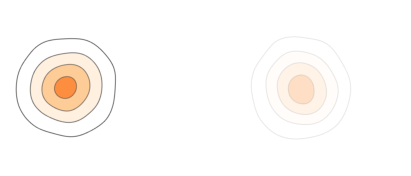
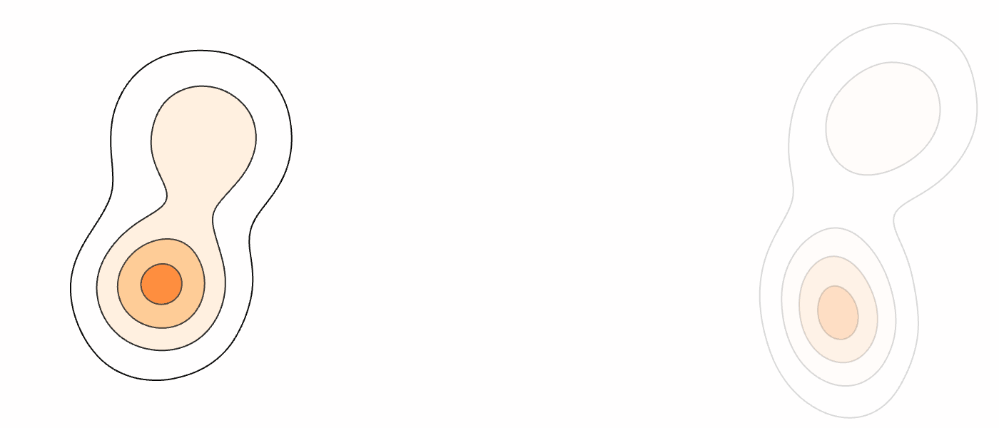
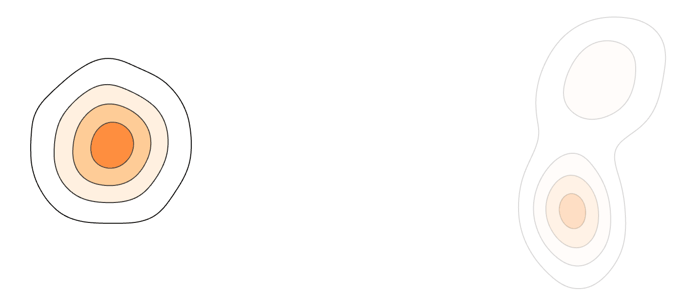
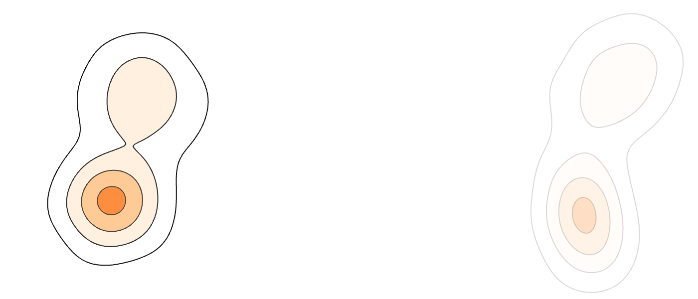
Motivation

Gaussian → Gaussian (Independent Coupling)

The classic flow matching paradigm where the target distribution (e.g., SD-VAE 1 latent space) is unimodal Gaussian.

GMM → GMM (Independent Coupling)

Estimate a data-adaptive mixture source distribution from the multimodal target distribution as a warm start.

Gaussian → GMM (Independent Coupling)

Paradigm shift to structured latent space (e.g., RAE 2, MAETok 3, SVGTok 4) that reduces the learning difficulty.

GMM → GMM (Mode Coupling)

Co-design with mode-dependent coupling achieves shortest and straightest sampling trajectories.

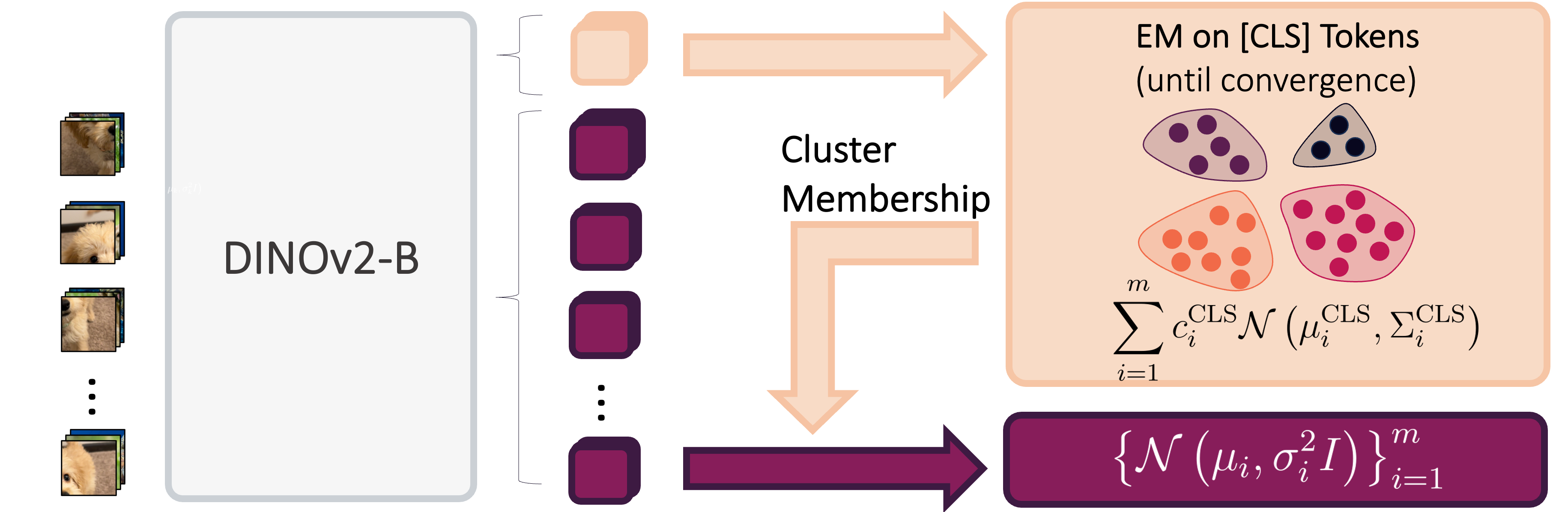
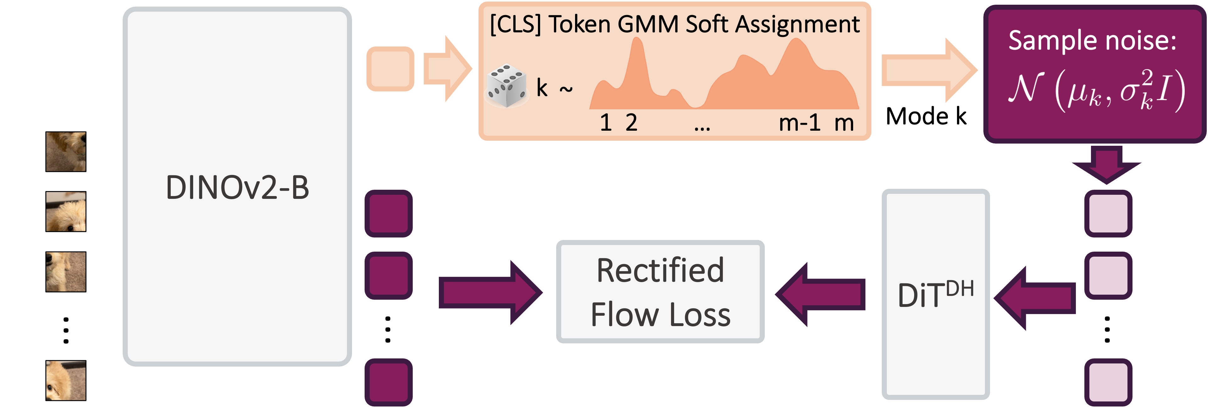
Our Method (MM-FM)

Our algorithm optimizes training efficiency by reducing learning difficulty through three key ideas: (1) employing a vision foundation model (DINOv2-B) as the visual tokenizer to reveal the union-of-manifold structure21 of the data; (2) fitting a GMM to the multimodal target distribution as a warm-start source distribution \(p = \sum_{i=1}^m c_i\mathcal{N}(\mu_i, \Sigma_i)\); and (3) designing a mode coupling \(\pi_{\textrm{mode}}(z_0 \mid z_1)\) that pairs each target sample with a source sample drawn from the nearest GMM mode, enabling local transport of probability mass.

▼

1

Stage 1: GMM Fitting

Figure 2: Fit a GMM to the foundation model encoded latents using EM on [CLS] tokens from DINOv2-B, then apply cluster membership to estimate the mean and covariance of each cluster on patch tokens (latents).

2

Stage 2: Flow Matching Training

Figure 3: The Flow Matching training process on the latent (patch tokens) by using pre-trained [CLS] GMM for mode assignment and sampling mode-dependent noise.

Experimental Results

On ImageNet256 dataset, without any conditioning (i.e., learning a purely unconditional velocity field), MM-FM (FID=3.82) without guidance outperforms the baseline using Gaussian source distribution and independent coupling (FID=9.33) on 80 epochs. It also outperforms the unconditional generation result (FID=4.96) with guidance on 200 epochs reported in RAE2.

Comparing with unconditional generation systems (i.e., without using annotated class labels) without guidance, MM-FM with mode conditioning (FID=3.18) on 80 epochs outperforms DLC16 with DLC conditioning (FID=5.75) on 80 epochs and RCG15 with MoCov3 conditioning (FID=4.89) on 400 epochs.

Though not relying on annotated class labels, MM-FM delivers matching and superior performance comparing with class-conditioning systems (including E2E-VAE11, VA-VAE12, MAETok3, AlignTok13, VFM-VAE14, and SVGTok4) in early checkpoints.

With AutoGuidance17, MM-FM trained for 80 epochs only without using annotated class labels achieves state-of-the-art FID=2.74 generation performance on ImageNet256.

Figure 4: FID vs. number of ODE steps for sampling (80 epochs).

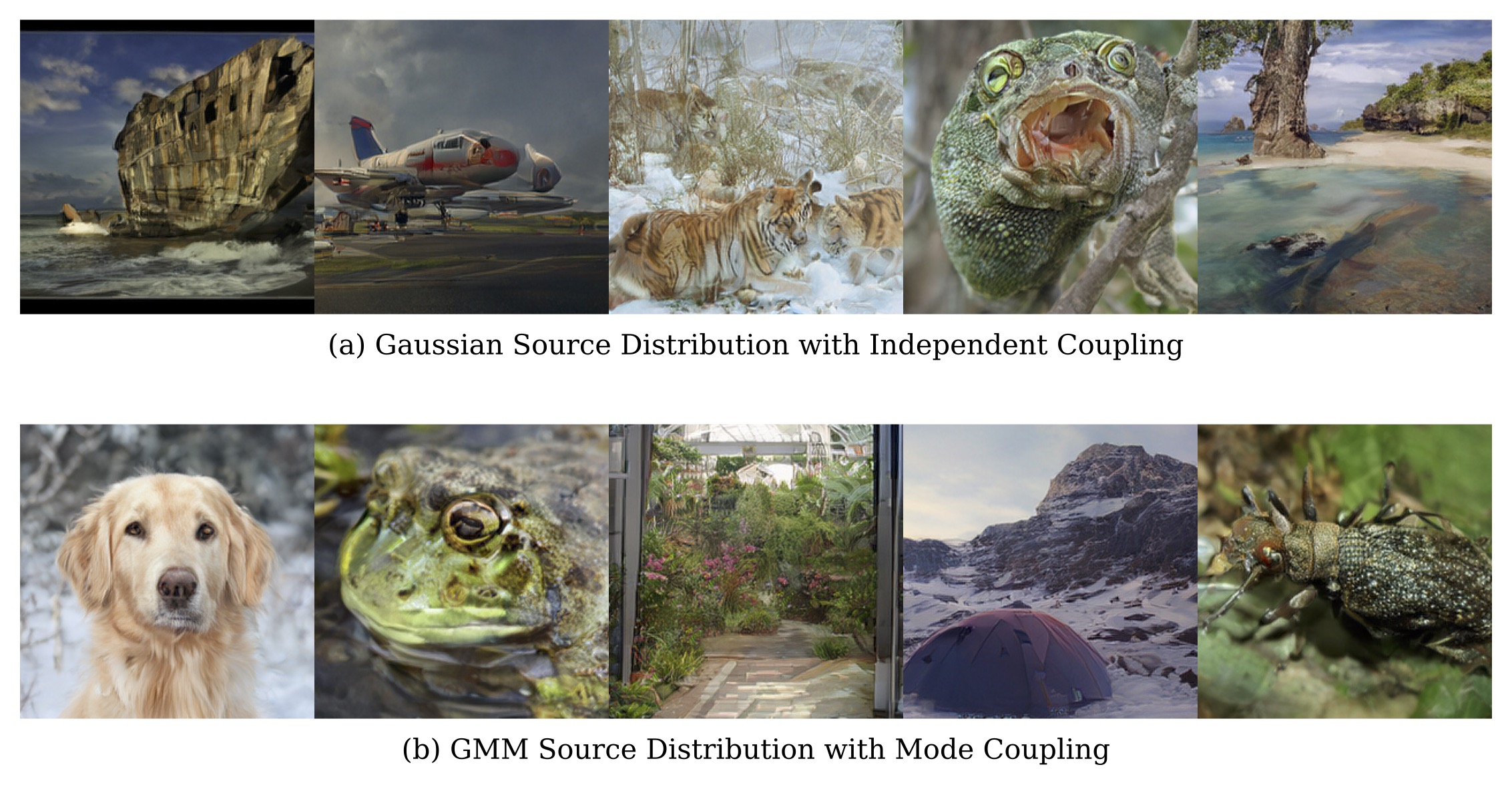
Besides training efficiency, MM-FM achieves inference efficiency due to reduced crossing of flows during training time. As a result, it has straighter sampling trajectories and thus requires fewer Euler steps of an ODE sampler. Figure 4 shows that MM-FM requires approximately 5x fewer steps to achieve comparable generation quality relative to Gaussian source distribution with independent coupling.

Ablation Study of GMM Parameters

Figure 5: Ablation on # GMM modes (spherical covariance type, soft assignment without mode conditioning).

Table 2: Ablation study of covariance and assignment types (# mode=64, 20 epochs, with mode conditioning).

FID-50K ↓	Soft Assignment			Hard Assignment
	Spherical	Diagonal	Full	Diagonal
	11.09	10.44	10.11	10.67

Data Efficiency

Figure 6: The qualitative comparison of unconditional generation (50 ODE steps) without guidance between baseline and MM-FM (without mode conditioning) on 10% ImageNet256 trained for 800 epochs using DiT^DH-S. (a) FID=24.33 (b) FID=7.48

Ablation Study of Foundation Model Encoders

We ablate the choice of foundation model encoder used for GMM fitting. Table 4 compares DINOv2-B, SigLIP2-B, and MAE-B in terms of linear probing accuracy and downstream generation quality (FID-50K).

Main Theoretical Results

We analyze multimodal generation with matched mixture distributions:

Here \(\tilde{q}\) and \(\tilde{p}\) are unimodal base distributions (e.g., standard Gaussians), and the mixtures are formed by placing transformed copies at locations \(\mu_k\) with covariances \(\Sigma_k\). Both \(p\) and \(q\) share the same parameters \(\{\mu_k,\Sigma_k\}_{k=1}^{m}\).

We compare two coupling strategies: mode coupling \(\pi_{\text{mode}}\) (our approach, where each source mode \(p_k\) flows only to the corresponding target mode \(q_k\)) vs. independent coupling \(\pi_{\text{ind}}\) (standard approach, where source and target are sampled independently). We measure the complexity of the multimodal generation problem by:

For additional theoretical results and complete proofs, please refer to our paper.

Conclusion

We propose MM-FM, which leverages vision foundation models as encoders to reveal the union-of-manifold structures in the latent space, and co-designs a multimodal GMM source distribution and mode coupling to exploit these structures. It delivers faster convergence and superior generation performance compared to the classic flow matching recipe that stays on unimodal Gaussian and independent coupling. We wish it provides a principled flow design for the co-evolution of foundation models and generative models. As more foundation models emerge across domains, training flow-based generative models can be made efficient by MM-FM.

For curious readers, we recommend Flow Matching Guide, Rectified Flow Tutorial, and A Visual Introduction to Rectified Flows for flow matching basics. For the insights into structured latents and training efficiency, we also recommend SVG and RAE's project page.

Citation

If you find this work useful, please consider citing:

References

1. Esser et al. "Scaling rectified flow transformers for high-resolution image synthesis." ICML'24. [Paper]
2. Zheng et al. "Diffusion Transformers with Representation Autoencoders." ICLR'26. [Project Page]
3. Chen et al. "Masked Autoencoders Are Effective Tokenizers for Diffusion Models." ICML'25. [Paper]
4. Shi et al. "Latent Diffusion Model without Variational Autoencoder." ICLR'26. [Project Page]
5. Helbling, et al. "Diffusion Explorer: Interactive Exploration of Diffusion Models." IEEE VIS'25. [Demo]
6. Liu et al. "Flow Straight and Fast: Learning to Generate and Transfer Data with Rectified Flow." ICLR'23. [Tutorial]
7. Lee et al. "Minimizing trajectory curvature of ode-based generative models." ICML'23. [Paper]
8. Rombach et al. "High-Resolution Image Synthesis with Latent Diffusion Models." CVPR'22. [Paper]
9. Peebles et al. "Scalable Diffusion Models with Transformers." ICCV'23. [Project Page]
10. Ma et al. "SiT: Exploring Flow and Diffusion-based Generative Models with Scalable Interpolant Transformers." ECCV'24. [Project Page]
11. Leng et al. "REPA-E: Unlocking VAE for End-to-End Tuning of Latent Diffusion Transformers." ICCV'25. [Project Page]
12. Yao et al. "Reconstruction vs. Generation: Taming Optimization Dilemma in Latent Diffusion Models." CVPR'25. [Paper]
13. Chen et al. "Aligning Visual Foundation Encoders to Tokenizers for Diffusion Models." arXiv. [Project Page]
14. Bi et al. "Vision Foundation Models Can Be Good Tokenizers for Latent Diffusion Models." arXiv. [Paper]
15. Li et al. "Return of Unconditional Generation: A Self-supervised Representation Generation Method." NeurIPS'24. [Paper]
16. Lavoie et al. "Compositional Discrete Latent Code for High Fidelity, Productive Diffusion Models." NeurIPS'25. [Paper]
17. Karras et al. "Guiding a Diffusion Model with a Bad Version of Itself." NeurIPS'24. [Paper]
18. Issachar et al. "Designing a Conditional Prior Distribution for Flow-Based Generative Models." arXiv. [Paper]
19. Jia et al. "Structured Diffusion Models with Mixture of Gaussians as Prior Distribution." arXiv. [Paper]
20. Chen et al. "Gaussian Mixture Flow Matching Models." ICML'25. [Paper]
21. Brown et al. "Verifying the Union of Manifolds Hypothesis for Image Data." ICLR'23. [Paper]